Introduction to Stochastic Calculus

import numpy as np
import matplotlib.pyplot as plt
import seaborn as sns
from scipy import stats

# Set random seed for reproducibility
np.random.seed(42)

Stochastic calculus is a branch of mathematics that deals with processes involving randomness. Two fundamental concepts in stochastic processes are Markov processes and martingales. Let’s understand their key differences and properties.

Markov Processes

A Markov process is characterized by the “memoryless” property: the future state depends only on the present state, not on the past history. Mathematically, for any times \(t_1 < t_2 < ... < t_n < t\):

\[ P(X_t | X_{t_n}, X_{t_{n-1}}, ..., X_{t_1}) = P(X_t | X_{t_n}) \]

Key properties: 1. Only the current state matters for predicting future states 2. Past history provides no additional information 3. Transitions depend only on the current state

Martingales

A martingale is a process where the expected future value equals the current value, given all past information. This is different from the Markov property. A process can be: - Markov but not a martingale - A martingale but not Markov - Both or neither

For a martingale, we have: \[ E(X_t | \mathcal{F}_s) = X_s \quad \text{for all } s < t \]

where \(\mathcal{F}_s\) represents all information available up to time \(s\).

Example: Fair Game

A classic example of a martingale is a fair game where: - Your current wealth is \(X_t\) - No matter what happened in previous rounds - Your expected future wealth equals your current wealth

def simulate_processes(n_steps=1000, n_paths=3):
    """
    Simulate and compare different stochastic processes.
    """
    # Time points
    t = np.linspace(0, 1, n_steps)
    dt = t[1] - t[0]
    
    # Initialize figure
    fig, (ax1, ax2) = plt.subplots(1, 2, figsize=(15, 6))
    
    # Simulate Markov process (Ornstein-Uhlenbeck)
    theta = 1.0  # mean reversion rate
    mu = 0.0    # long-term mean
    sigma = 0.5  # volatility
    
    for _ in range(n_paths):
        X = np.zeros(n_steps)
        for i in range(1, n_steps):
            dX = theta * (mu - X[i-1]) * dt + sigma * np.sqrt(dt) * np.random.normal()
            X[i] = X[i-1] + dX
        ax1.plot(t, X, label=f'Path {_+1}')
    
    ax1.set_title('Markov Process\n(Ornstein-Uhlenbeck)')
    ax1.set_xlabel('Time')
    ax1.set_ylabel('Value')
    ax1.legend()
    ax1.grid(True)
    
    # Simulate Martingale (Geometric Brownian Motion with μ=0)
    sigma = 0.3
    
    for _ in range(n_paths):
        X = np.zeros(n_steps)
        X[0] = 1.0
        for i in range(1, n_steps):
            X[i] = X[i-1] * np.exp(-0.5*sigma**2*dt + sigma*np.sqrt(dt)*np.random.normal())
        ax2.plot(t, X, label=f'Path {_+1}')
    
    ax2.set_title('Martingale Process\n(Zero-drift GBM)')
    ax2.set_xlabel('Time')
    ax2.set_ylabel('Value')
    ax2.legend()
    ax2.grid(True)
    
    plt.tight_layout()
    plt.show()

# Simulate and visualize the processes
simulate_processes()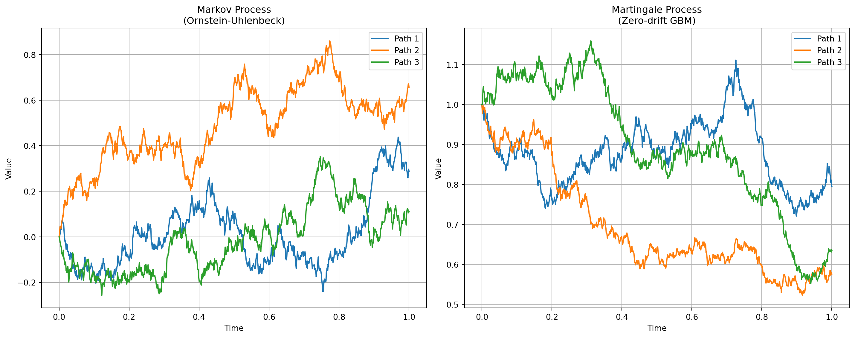

The Martingle property states that the expected value of the next period is the current period value

\[ E(X_i | X_j, j < i) = X_j \]

Quadratic Variation

Definition

The quadratic variation of a stochastic process \(X_t\) over an interval \([t_0, t_1]\) is defined as the limit of the sum of squared increments:

\[ [X,X]_{t_0}^{t_1} = \lim_{n \to \infty} \sum_{i=1}^{n} (X_{t_i} - X_{t_{i-1}})^2 \]

where the interval \([t_0, t_1]\) is partitioned into \(n\) subintervals with partition points \(t_0 < t_1 < ... < t_n = t_1\).

Properties

1. Finite Variation Processes:
   • For continuous processes of finite variation (e.g., differentiable functions)
   • Quadratic variation is zero
2. Brownian Motion:
   • For a standard Brownian motion \(W_t\)
   • \([W,W]_0^t = t\)
   • This is a fundamental property used in Itô calculus
3. Martingales:
   • For continuous martingales
   • Quadratic variation exists and is increasing
   • Used to characterize the “roughness” of paths

Financial Applications

Quadratic variation is crucial in finance for: 1. Measuring volatility 2. Option pricing 3. Risk management 4. Volatility forecasting

The realized variance in financial markets is an empirical estimate of quadratic variation.

def compute_quadratic_variation(X, t):
    """
    Compute the quadratic variation of a process X.
    
    Parameters:
    -----------
    X : array_like
        Process values
    t : array_like
        Time points
        
    Returns:
    --------
    qv : array_like
        Cumulative quadratic variation
    """
    increments = np.diff(X)
    qv = np.cumsum(increments**2)
    return np.concatenate(([0], qv))

def simulate_and_analyze_qv(T=1.0, n_steps=1000):
    """
    Simulate processes and analyze their quadratic variation.
    """
    # Time grid
    t = np.linspace(0, T, n_steps)
    dt = t[1] - t[0]
    
    # Parameters
    sigma = 0.2  # volatility
    
    # Initialize processes
    W = np.zeros(n_steps)  # Brownian motion
    S = np.zeros(n_steps)  # Smooth process
    
    # Simulate paths
    for i in range(1, n_steps):
        # Brownian motion
        W[i] = W[i-1] + np.sqrt(dt) * np.random.normal()
        
        # Smooth process (sine wave)
        S[i] = np.sin(2*np.pi*t[i])
    
    # Compute quadratic variations
    qv_W = compute_quadratic_variation(W, t)
    qv_S = compute_quadratic_variation(S, t)
    
    # Plotting
    fig, ((ax1, ax2), (ax3, ax4)) = plt.subplots(2, 2, figsize=(15, 10))
    
    # Plot processes
    ax1.plot(t, W, label='Brownian Motion')
    ax1.plot(t, S, label='Smooth Process')
    ax1.set_title('Sample Paths')
    ax1.set_xlabel('Time')
    ax1.set_ylabel('Value')
    ax1.legend()
    ax1.grid(True)
    
    # Plot increments
    ax2.hist(np.diff(W), bins=50, alpha=0.5, label='BM Increments')
    ax2.hist(np.diff(S), bins=50, alpha=0.5, label='Smooth Increments')
    ax2.set_title('Distribution of Increments')
    ax2.set_xlabel('Increment Size')
    ax2.set_ylabel('Frequency')
    ax2.legend()
    
    # Plot quadratic variations
    ax3.plot(t, qv_W, label='Brownian Motion')
    ax3.plot(t, t, '--', label='Theoretical (t)')
    ax3.set_title('Quadratic Variation of Brownian Motion')
    ax3.set_xlabel('Time')
    ax3.set_ylabel('Quadratic Variation')
    ax3.legend()
    ax3.grid(True)
    
    ax4.plot(t, qv_S, label='Smooth Process')
    ax4.set_title('Quadratic Variation of Smooth Process')
    ax4.set_xlabel('Time')
    ax4.set_ylabel('Quadratic Variation')
    ax4.legend()
    ax4.grid(True)
    
    plt.tight_layout()
    plt.show()
    
    # Print analysis
    print("\nQuadratic Variation Analysis:")
    print(f"Brownian Motion final QV: {qv_W[-1]:.4f} (should be ≈ {T:.4f})")
    print(f"Smooth Process final QV: {qv_S[-1]:.4f} (should be ≈ 0)")

# Run simulation
simulate_and_analyze_qv()

Quadratic Variation Analysis:
Brownian Motion final QV: 1.0539 (should be ≈ 1.0000)
Smooth Process final QV: 0.0198 (should be ≈ 0)

Stochastic Integration

Introduction

Stochastic integration extends the concept of integration to handle random processes. The most important type is the Itô integral, which is defined for stochastic processes with respect to Brownian motion.

The Itô Integral

For a stochastic process \(H_t\), the Itô integral with respect to Brownian motion \(W_t\) is denoted as:

\[ \int_0^t H_s dW_s = \lim_{n \to \infty} \sum_{i=1}^n H_{t_{i-1}}(W_{t_i} - W_{t_{i-1}}) \]

Key properties: 1. Martingale Property: The Itô integral is a martingale 2. Isometry: \(\mathbb{E}\left[\left(\int_0^t H_s dW_s\right)^2\right] = \mathbb{E}\left[\int_0^t H_s^2 ds\right]\) 3. Zero Mean: \(\mathbb{E}\left[\int_0^t H_s dW_s\right] = 0\)

Differences from Riemann Integration

1. Choice of Evaluation Point:
   • Riemann: Can evaluate at any point in interval
   • Itô: Must evaluate at left endpoint (non-anticipating)
2. Path Properties:
   • Riemann: Works for smooth paths
   • Itô: Works for continuous but nowhere differentiable paths
3. Chain Rule:
   • Riemann: Standard calculus rules apply
   • Itô: Additional term appears (Itô’s lemma)

def simulate_ito_integral(T=1.0, n_steps=1000, n_paths=1000):
    """
    Simulate Itô integrals for different integrands.
    """
    # Time grid
    t = np.linspace(0, T, n_steps)
    dt = t[1] - t[0]
    
    # Initialize arrays for different integrals
    I1 = np.zeros(n_paths)  # ∫ t dW_t
    I2 = np.zeros(n_paths)  # ∫ W_t dW_t
    
    # Simulate multiple paths
    for path in range(n_paths):
        # Simulate Brownian motion
        dW = np.sqrt(dt) * np.random.normal(size=n_steps-1)
        W = np.cumsum(np.concatenate(([0], dW)))
        
        # Compute Itô integrals
        # 1. ∫ t dW_t
        I1[path] = np.sum(t[:-1] * dW)
        
        # 2. ∫ W_t dW_t
        I2[path] = np.sum(W[:-1] * dW)
    
    # Theoretical results
    # For ∫ t dW_t: mean = 0, variance = T^3/3
    # For ∫ W_t dW_t: equals W_T^2/2 - T/2 (Itô's formula)
    
    # Plotting
    fig, (ax1, ax2) = plt.subplots(1, 2, figsize=(15, 6))
    
    # Plot distribution of ∫ t dW_t
    sns.histplot(data=I1, stat='density', ax=ax1)
    x = np.linspace(min(I1), max(I1), 100)
    theoretical_pdf = stats.norm.pdf(x, 0, np.sqrt(T**3/3))
    ax1.plot(x, theoretical_pdf, 'r-', label='Theoretical')
    ax1.set_title('Distribution of $\\int_0^T t\\,dW_t$')
    ax1.set_xlabel('Value')
    ax1.set_ylabel('Density')
    ax1.legend()
    
    # Plot distribution of ∫ W_t dW_t
    sns.histplot(data=I2, stat='density', ax=ax2)
    ax2.set_title('Distribution of $\\int_0^T W_t\\,dW_t$')
    ax2.set_xlabel('Value')
    ax2.set_ylabel('Density')
    
    plt.tight_layout()
    plt.show()
    
    # Print analysis
    print("\nItô Integral Analysis:")
    print("\n1. ∫ t dW_t")
    print(f"Sample Mean: {np.mean(I1):.4f} (Theory: 0)")
    print(f"Sample Variance: {np.var(I1):.4f} (Theory: {T**3/3:.4f})")
    
    print("\n2. ∫ W_t dW_t")
    print(f"Sample Mean: {np.mean(I2):.4f}")
    print(f"Sample Variance: {np.var(I2):.4f}")

# Run simulation
simulate_ito_integral()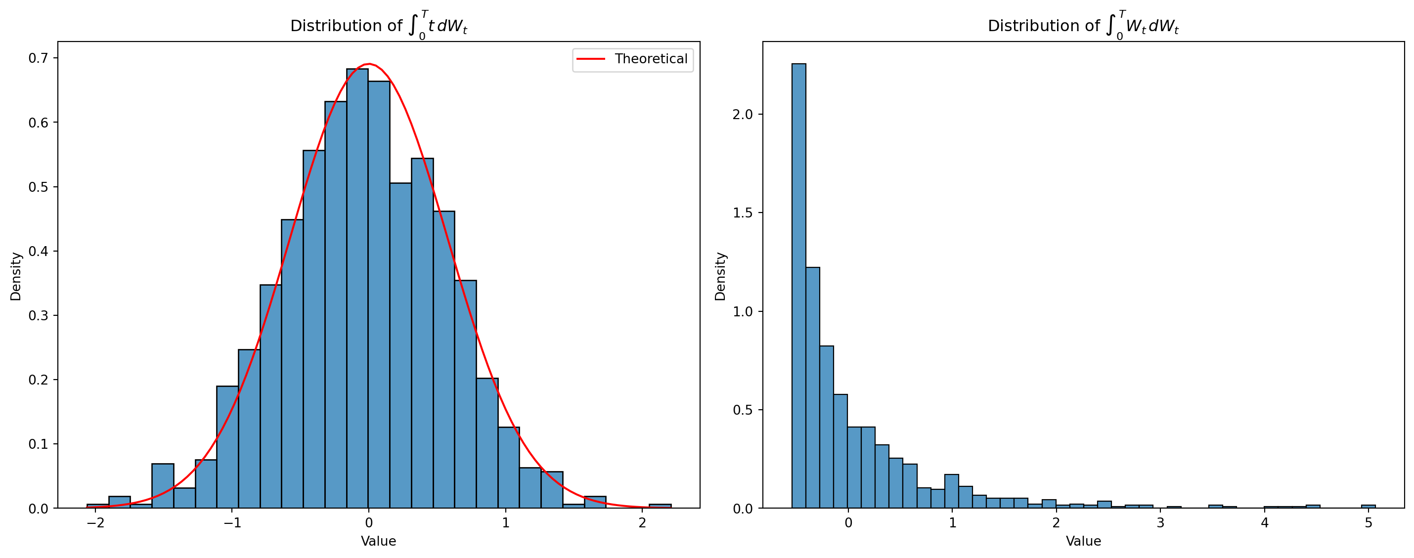

Itô Integral Analysis:

1. ∫ t dW_t
Sample Mean: -0.0405 (Theory: 0)
Sample Variance: 0.3525 (Theory: 0.3333)

2. ∫ W_t dW_t
Sample Mean: 0.0415
Sample Variance: 0.5623

Stochastic Differential Equations (SDEs)

Introduction

A stochastic differential equation (SDE) is a differential equation where one or more terms involve a stochastic process. The general form is:

\[ dX_t = a(X_t, t)dt + b(X_t, t)dW_t \]

where: - \(a(X_t, t)\) is the drift coefficient - \(b(X_t, t)\) is the diffusion coefficient - \(W_t\) is a Brownian motion

Common Examples

1. Geometric Brownian Motion (Black-Scholes model): \[ dS_t = \mu S_t dt + \sigma S_t dW_t \]

2. Ornstein-Uhlenbeck Process (Mean-reverting): \[ dX_t = \theta(\mu - X_t)dt + \sigma dW_t \]

3. Cox-Ingersoll-Ross Process (Interest rates): \[ dr_t = \kappa(\theta - r_t)dt + \sigma\sqrt{r_t}dW_t \]

Numerical Solutions

SDEs are typically solved using numerical methods:

1. Euler-Maruyama Method: \[ X_{t+\Delta t} = X_t + a(X_t, t)\Delta t + b(X_t, t)\sqrt{\Delta t}Z \] where \(Z \sim \mathcal{N}(0,1)\)

2. Milstein Method (Higher order): \[ X_{t+\Delta t} = X_t + a\Delta t + b\Delta W + \frac{1}{2}b\frac{\partial b}{\partial x}[(\Delta W)^2 - \Delta t] \]

Applications in Finance

1. Asset price modeling
2. Interest rate dynamics
3. Volatility processes
4. Credit risk modeling
5. Option pricing

def simulate_sde(sde_type='gbm', T=1.0, n_steps=1000, n_paths=5):
    """
    Simulate different types of SDEs using Euler-Maruyama method.
    
    Parameters:
    -----------
    sde_type : str
        Type of SDE to simulate ('gbm', 'ou', or 'cir')
    T : float
        Time horizon
    n_steps : int
        Number of time steps
    n_paths : int
        Number of paths to simulate
    """
    # Time grid
    t = np.linspace(0, T, n_steps)
    dt = t[1] - t[0]
    
    # Initialize arrays
    X = np.zeros((n_paths, n_steps))
    
    # Set parameters based on SDE type
    if sde_type == 'gbm':  # Geometric Brownian Motion
        mu = 0.1    # drift
        sigma = 0.2  # volatility
        X[:, 0] = 1.0  # initial value
        title = 'Geometric Brownian Motion'
        
    elif sde_type == 'ou':  # Ornstein-Uhlenbeck
        theta = 1.0  # mean reversion rate
        mu = 0.0    # long-term mean
        sigma = 0.3  # volatility
        X[:, 0] = 0.0
        title = 'Ornstein-Uhlenbeck Process'
        
    else:  # Cox-Ingersoll-Ross
        kappa = 1.0  # mean reversion rate
        theta = 0.05  # long-term mean
        sigma = 0.2  # volatility
        X[:, 0] = 0.05
        title = 'Cox-Ingersoll-Ross Process'
    
    # Simulate paths
    for i in range(n_paths):
        for j in range(1, n_steps):
            dW = np.sqrt(dt) * np.random.normal()
            
            if sde_type == 'gbm':
                X[i, j] = X[i, j-1] * (1 + mu*dt + sigma*dW)
                
            elif sde_type == 'ou':
                X[i, j] = X[i, j-1] + theta*(mu - X[i, j-1])*dt + sigma*dW
                
            else:  # CIR
                X[i, j] = X[i, j-1] + kappa*(theta - X[i, j-1])*dt + sigma*np.sqrt(max(X[i, j-1], 0))*dW
    
    # Plotting
    plt.figure(figsize=(12, 6))
    
    # Plot sample paths
    for i in range(n_paths):
        plt.plot(t, X[i], alpha=0.7, label=f'Path {i+1}')
    
    # Add theoretical properties
    if sde_type == 'gbm':
        # Plot theoretical mean
        theory_mean = X[0, 0] * np.exp(mu * t)
        plt.plot(t, theory_mean, 'k--', label='Theoretical Mean')
        
    elif sde_type == 'ou':
        # Plot mean reversion level
        plt.axhline(y=mu, color='k', linestyle='--', label='Mean Level')
        
    else:  # CIR
        plt.axhline(y=theta, color='k', linestyle='--', label='Long-term Mean')
    
    plt.title(title)
    plt.xlabel('Time')
    plt.ylabel('Value')
    plt.legend()
    plt.grid(True)
    plt.show()

# Simulate all three types of SDEs
print("1. Geometric Brownian Motion (GBM)")
simulate_sde('gbm')

print("\n2. Ornstein-Uhlenbeck Process")
simulate_sde('ou')

print("\n3. Cox-Ingersoll-Ross Process")
simulate_sde('cir')

1. Geometric Brownian Motion (GBM)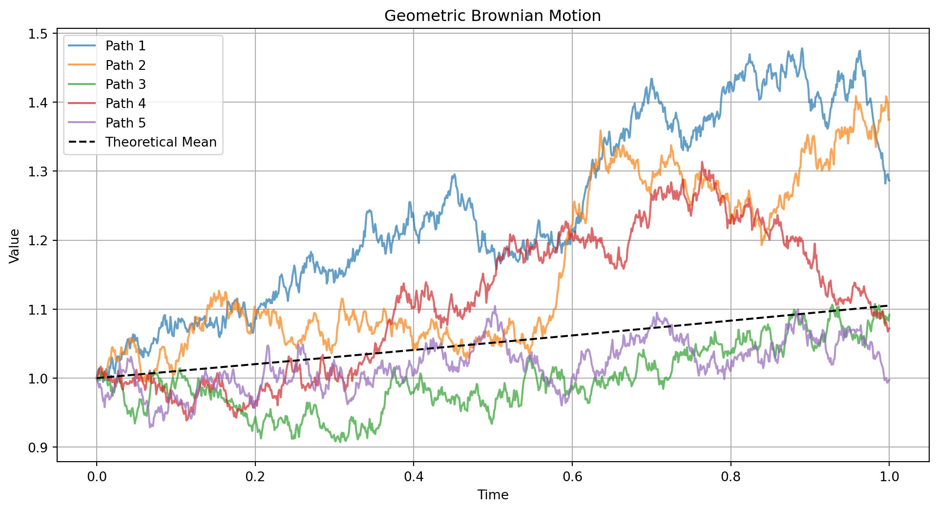

2. Ornstein-Uhlenbeck Process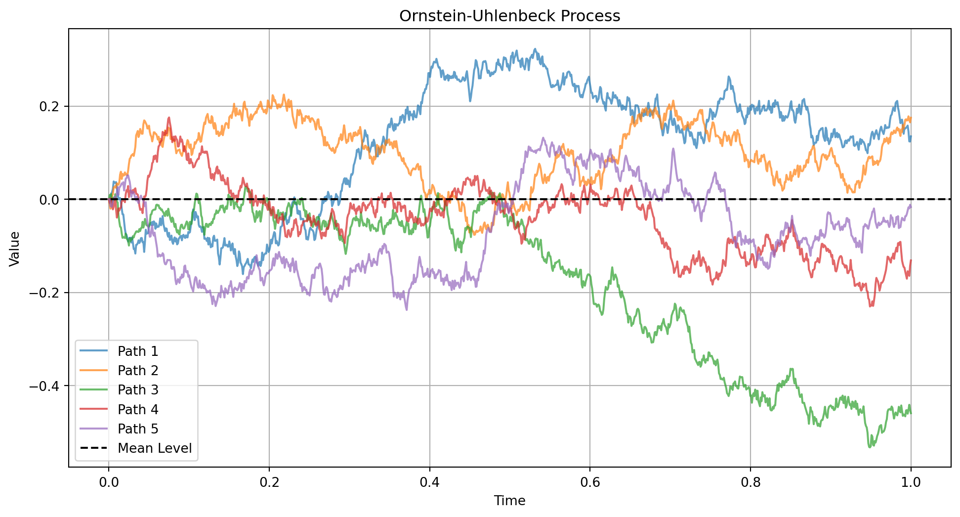

3. Cox-Ingersoll-Ross Process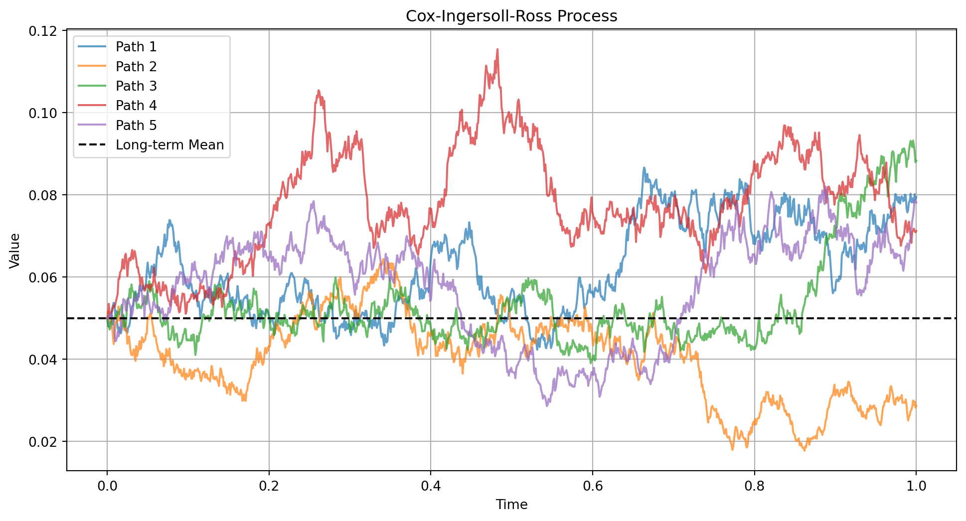

Summary and Key Concepts

In this chapter, we’ve covered the fundamental concepts of stochastic calculus:

1. Markov and Martingale Properties

• Markov property: Future depends only on present
• Martingale property: Expected future value equals present value
• These properties can exist independently

2. Quadratic Variation

• Measures cumulative variability of a process
• Key difference between stochastic and ordinary calculus
• Brownian motion has quadratic variation equal to time

3. Stochastic Integration

• Itô integral extends integration to random processes
• Different from Riemann integration
• Forms basis for stochastic calculus

4. Stochastic Differential Equations

• Model random processes with differential equations
• Common models: GBM, OU, CIR processes
• Solved numerically using Euler-Maruyama method

Applications in Finance

1. Asset Pricing:
   • Stock price modeling (GBM)
   • Option pricing (Black-Scholes)
2. Risk Management:
   • Interest rate modeling (CIR)
   • Volatility modeling
3. Portfolio Theory:
   • Portfolio optimization
   • Risk assessment

Next Steps

The next chapter will build on these concepts to develop the Black-Scholes option pricing model, which is a cornerstone of modern financial theory.